
Genetic Dissection of Complex Traits
Abstract
Medical genetics was revolutionized during the 1980s by the application of genetic mapping to locate the genes responsible for simple Mendelian diseases. Most diseases and traits, however, do not follow simple inheritance patterns. Geneticists have thus begun taking up the even greater challenge of the genetic dissection of complex traits. Four major approaches have been developed: linkage analysis, allele-sharing methods, association studies, and polygenic analysis of experimental crosses. This article synthesizes the current state of the genetic dissection of complex traits—describing the methods, limitations, and recent applications to biological problems.
Human genetics has sparked a revolution in medical science on the basis of the seemingly improbable notion that one can systematically discover the genes causing inherited diseases without any prior biological clue as to how they function. The method of genetic mapping, by which one compares the inheritance pattern of a trait with the inheritance patterns of chromosomal regions, allows one to find where a gene is without knowing what it is. The approach is completely generic, being equally applicable to spongiform brain degeneration as to inflammatory bowel disease.
To geneticists, this revolution is really nothing new. Genetic mapping of trait-causing genes to chromosomal locations dates back to the work of Sturtevant in 1913 (1). It has been a mainstay of experimental geneticists who study fruit flies, nematode worms, yeast, and maize and who developed genetic maps containing hundreds of genetic markers that made it possible to follow the inheritance of any chromosomal region in a controlled cross. With the advent of recombinant DNA, genetic mapping was carried to its logical conclusion with the development of positional cloning-the isolation of a gene solely on the basis of its chromosomal location, without regard to its biochemical function. Positional cloning was invented by Bender and colleagues, who used it to isolate the bithorax complex in Drosophila (2), and it rapidly became a routine technique in flies and worms.
Despite its central role in experimental organisms, genetic mapping hardly figured in the study of humans throughout most of the century. There were two reasons: the lack of an abundant supply of genetic markers with which to study inheritance, and the inability to arrange human crosses to suit experimental purposes. The key breakthrough was the recognition that naturally occurring DNA sequence variation provided a virtually unlimited supply of genetic markers-an idea first conceived of by Botstein and colleagues for yeast crosses (3) and subsequently for human families (4). With highly polymorphic genetic markers, one could trace inheritance in existing human pedigrees as if one had set up the crosses in the laboratory. These ideas soon led to an explosion of interest in the genetic mapping of rare human diseases having simple Mendelian inheritance. More than 400 such diseases have been genetically mapped in this manner, and nearly 40 have been positionally cloned (5).
Human geneticists are now beginning to explore a new genetic frontier, driven by an inconvenient reality: Most traits of medical relevance do not follow simple Mendelian monogenic inheritance. Such “complex” traits include susceptibilities to heart disease, hypertension, diabetes, cancer, and infection. The genetic dissection of complex traits is attracting many investigators with the promise of shedding light on old problems and is spawning a variety of analytical methods. The emerging issues turn out to be relevant not just to medical genetics, but to fundamental studies of mammalian development and applied work in agricultural improvement. The field is still at an early stage, but it is ready to explode much as it has done in recent years with the analysis of simple traits. The purpose of this article is to synthesize the key challenges and methods, to highlight some enlightening examples, and to identify further needs.
Complex traits
The term “complex trait” refers to any phenotype that does not exhibit classic Mendelian recessive or dominant inheritance attributable to a single gene locus. In general, complexities arise when the simple correspondence between genotype and phenotype breaks down, either because the same genotype can result in different phenotypes (due to the effects of chance, environment, or interactions with other genes) or different genotypes can result in the same phenotype.
To some extent, the category of complex traits is all-inclusive. Even the simplest genetic disease is complex, when looked at closely. Sickle cell anemia is a classic example of a simple Mendelian recessive trait. Yet, individuals carrying identical alleles at the β-globin locus can show markedly different clinical courses, ranging from early childhood mortality to a virtually unrecognized condition at age 50 (6). The trait of severe sickle cell anemia is thus complex, being influenced by multiple genetic factors including a mapped X-linked locus and an inferred autosomal locus that can increase fetal hemoglobin amounts and thereby partially ameliorate the disease (7).
It is often impossible to find a genetic marker that shows perfect cosegregation with a complex trait. The reasons for this can be ascribed to a few basic problems.
Incomplete penetrance and phenocopy.
Some individuals who inherit a predisposing allele may not manifest the disease (incomplete penetrance), whereas others who inherit no predisposing allele may nonetheless get the disease as a result of environmental or random causes (phenocopy). Thus, the genotype at a given locus may affect the probability of disease, but not fully determine the outcome. The penetrance function f(G), specifying the probability of disease for each genotype G, may also depend on nongenetic factors such as age, sex, environment, and other genes. For example, the risk of breast cancer by ages 40, 55, and 80 is 37%, 66%, and 85% in a woman carrying a mutation at the BRCA1 locus as compared with 0.4%, 3%, and 8% in a noncarrier (8). In such cases, genetic mapping is hampered by the fact that a predisposing allele may be present in some unaffected individuals or absent in some affected individuals.
Genetic (or locus) heterogeneity.
Mutations in any one of several genes may result in identical phenotypes, such as when the genes are required for a common biochemical pathway or cellular structure. This poses no problem in experimental organisms, because geneticists can arrange to work with pure-breeding strains and perform crosses to assign mutations to complementation classes. In contrast, medical geneticists typically have no way to know whether two patients suffer from the same disease for different genetic reasons, at least until the genes are mapped. Examples of genetic heterogeneity in humans include polycystic kidney disease (9), early-onset Alzheimer’s disease (10), maturity-onset diabetes of the young (11), hereditary nonpolyposis colon cancer (12), ataxia telangiectasia (13), and xeroderma pigmentosum (14). Retinitis pigmentosa, involving retinal degeneration, apparently can result from mutations in any of at least 14 different loci (15), and Zellweger syndrome, involving the failure of peroxisome biosynthesis, from mutations in any of 13 loci (16). Genetic heterogeneity hampers genetic mapping, because a chromosomal region may cosegregate with a disease in some families but not in others. Genetic heterogeneity should be distinguished from allelic heterogeneity, in which there are multiple disease-causing mutations at a single gene. Allelic heterogeneity tends not to interfere with gene mapping.
Polygenic inheritance.
Some traits may require the simultaneous presence of mutations in multiple genes. Polygenic traits may be classified as discrete traits, measured by a specific outcome (for example, development of type I diabetes or death from myocardial infarction), or quantitative traits, measured by a continuous variable [for example, diastolic blood pressure, fasting glucose concentrations, or immunoglobulin E (IgE) titers] whose level may be set by the combined action of individual quantitative trait loci. Discrete traits may represent a threshold effect, produced whenever an underlying quantitative variable, influenced by multiple genes, exceeds a critical threshold, or a pure synthetic effect, requiring the simultaneous and joint action of each of several mutations.
Polygenic inheritance is easily demonstrated in animal crosses, in the transmission pattern of quantitative traits such as blood pressure (17), and in the pervasive “genetic background” effects that represent the action of modifier genes. For example, a mutation in the mouse Apc gene causes numerous intestinal neoplasias and early death in B6 mice but has barely noticeable effects when bred into an AKR strain (18). More generally, the phenotype of “knockout mice” may vary dramatically on different strain backgrounds, pointing to previously unknown interacting genes.
Polygenic inheritance is harder to demonstrate directly in humans, but it is surely no less common. One form of retinitis pigmentosa was shown to be due to strict digenic inheritance, requiring the presence of heterozygous mutations at the peripherin/ RDS and ROMI genes (19) (whose encoded proteins are thought to interact in the photoreceptor outer segment disc membranes). Some forms of Hirschsprung disease appear to require the simultaneous presence of mutations on chromosomes 13, 21, and possibly elsewhere (20). Polygenic inheritance complicates genetic mapping, because no single locus is strictly required to produce a discrete trait or a high value of a quantitative trait [except in the case of a pure synthetic interaction causing a discrete trait (21, 22)].
High frequency of disease-causing alleles.
Even a simple trait can be hard to map if disease-causing alleles D occur at high frequency in the population. The expected Mendelian inheritance pattern of disease will be confounded by the problem that multiple independent copies of D may be segregating in the pedigree [often referred to as bi-lineality (23)] and that some individuals may be homozygous for D [in which case one will not observe linkage between D and a specific allele at a nearby genetic marker, because either of the two homologous chromosomes could be passed to an affected offspring (24)]. Late-onset Alzheimer’s disease provides an excellent example. Initial linkage studies found weak evidence of linkage to chromosome 19q, but they were dismissed by many observers because the lod score (logarithm of the likelihood ratio for linkage) remained relatively low, and it was difficult to pinpoint the linkage with any precision (25). The confusion was finally resolved with the discovery that the apolipoprotein E type 4 allele appears to be the major causative factor on chromosome 19. The high frequency of the allele (~16% in most populations) had interfered with the traditional linkage analysis (26). High frequency of disease-causing alleles becomes an even greater problem if genetic heterogeneity is also present.
Other transmission mechanisms.
Finally, mammalian genetics has revealed additional modes of genetic inheritance. These include mitochondrial inheritance (in which mitochondria pass solely through the material germ line, and each meiotic transmission may involve selection from a potentially mixed population of mutant and normal organelles); imprinting (due to differential activity of the paternal and maternal copies of a gene); and phenomena due to the expansion of trinucleotide repeats such as so-called “anticipation.” These modes of transmission pose little difficulty when they obey strict rules (as for imprinting), but they can complicate analysis when they lead to highly variable transmission rates [as for some mitochondrial diseases or trinucleotide repeat diseases (27)] and may require specialized methods (28).
Genetic epidemiology
Before undertaking DNA-based studies aimed at genetic dissection, one would ideally like to infer as much as possible about the genetic basis of a trait on the basis of the pattern of disease incidence in families and populations. Such genetic epidemiology constitutes a major field in its own right for which excellent reviews exist (29). We focus on a few key concepts.
Twin studies.
Whereas experimental geneticists can propagate inbred lines with isogenic genetic constitution, the only opportunity to examine the expression of a human trait in a fixed genetic background comes from the study of monozygotic (MZ) twins (30). The absolute risk to an MZ twin of an affected individual provides a direct estimate of penetrance for a given environment.
Relative risk.
The most important epidemiological parameter is the relative risk, λR, defined as the recurrence risk for a relative of an affected person divided by the risk for the general population. The subscript R denotes the type of relation; for example, λO and λS are the risks to offspring and sibs, respectively. The magnitude of λR is related to the degree of concordant inheritance for genetic determinants in affected relative pairs and thus is related to the ease or difficulty of genetic mapping, as shown by Risch (31–33). Genetic mapping is much easier for traits with high λ (for example, λS > 10) than for those with low λ (for example, λS < 2). As an illustration of the range, λS ≈ 500 for cystic fibrosis; 15 for type I diabetes [of which a factor of 3 to 4 is attributable to concordance at the human leukocyte antigen (HLA) complex]; 8.6 for schizophrenia; and 3.5 for type II diabetes. For a quantitative phenotype, a similar measure is the heritability of the trait (34).
Segregation analysis.
Segregation analysis involves fitting a general model to the inheritance pattern of a trait in pedigrees. Using a model involving the presence of a simple Mendelian factor in a background of multifactorial inheritance, one tries to estimate key parameters such as the allele frequency, penetrance, and proportion of cases explained by the Mendelian factor. An important example is the work of Newman et al. and other researchers (35, 36) who showed that the degree of familial clustering for breast cancer observed in 1579 nuclear families was consistent with a dominantly acting rare allele (frequency = 0.06%), accounting for 4% of affected women (but 20% of affected mother-daughter pairs), in a larger background of multifactorial causation. Segregation analysis can be extremely sensitive to biases in the ascertainment of families [for example, if preferential inclusion of affected individuals may cause the penetrance to be greatly overstated (37)], and it may have little ability to distinguish among the many possible modes of inheritance for complex traits (38). Moreover, it can be especially difficult to estimate the number of distinct genes influencing a trait, except in very favorable situations (39), and to identify penetrance parameters associated with multiple loci (40).
Defining diseases
Given the many problems that can hamper genetic dissection of complex traits, geneticists try to stack the deck in their favor. By narrowing the definition of a disease or restricting the patient population, it is often possible to work with a trait that is more nearly Mendelian in its inheritance pattern and more likely to be homogeneous. The extent to which redefinition simplifies the task of genetic mapping can be measured by the resulting increase in the relative risk λR. Although there is no guaranteed method to increase λR, four criteria are often useful.
Clinical phenotype.
For example, when colon cancer is restricted to cases with extreme polyposis, the trait becomes a simple autosomal dominant one which allowed positional cloning of the APC gene on chromosome 5 (41). Other forms of colon cancer can be distinguished by the phenotype of replication errors in tumors (42). In studying hypertension, one can increase λ by focusing on cases with combined hypertension and hyperlipidemia (43).
Age at onset.
Breast cancer and Alzheimer’s disease are rendered genetically more homogeneous by focusing on early-onset cases [although the latter can be caused by at least three independent loci (44)]. Similarly, the relative risk for death from heart attack is much greater for early-onset cases (λS ≈ 7 in men and ≈15 in women under age 65) as compared with late-onset cases (λS ≈ 2) (45).
Family history.
For example, the sister of a woman with breast cancer has a much greater risk if her mother is also affected (35, 36). Hereditary nonpolyposis colon cancer (12) was genetically mapped by defining the trait to require the presence of at least two other affected relatives.
Severity.
For continuous traits, it often pays to consider as affected only those individuals at the extreme ends of the trait distribution. For example, one might select families for a hypertension study on the basis of the presence of at least one member with blood pressure exceeding 140/90. Such selection can greatly increase the ability to map genes, both in human families (46) and experimental crosses (47).
Another way to improve the prospects for genetic dissection is to focus on specific ethnic groups. Population genetic theory and data suggest that there will be greater genetic and allelic homogeneity in a more genetically isolated group (such as Sardinians, Basques, Finns, and Japanese) than in a large, mixed population (such as is in New York City or Los Angeles). Different ethnic groups may shed light on different aspects of a disease, which might be much harder to discern in an outbred population. For example, it has been suggested that there may be differences in the genetic etiology of type II diabetes between Mexican Americans and Scandinavians, with somewhat higher frequency of early insulin resistance in the former and an early pancreatic beta cell defect in the latter (48). Focusing on a highly restricted population may also offer advantages for eventual positional cloning, because one may be able to exploit linkage disequilibrium for fine-structure genetic mapping (discussed below).
Genetic dissection: the fourfold way
The methods available for genetic dissection of complex traits fall neatly into four categories: linkage analysis, allele-sharing methods, association studies in human populations, and genetic analysis of large crosses in model organisms such as the mouse and rat.
Linkage analysis
Linkage analysis involves proposing a model to explain the inheritance pattern of phenotypes and genotypes observed in a pedigree (Fig. 1). It is the method of choice for simple Mendelian traits because the allowable models are few and easily tested. However, applications to complex traits can be more problematic, because it may be hard to find a precise model that adequately explains the inheritance pattern.
Formally, linkage analysis consists of finding a model M1, positing a specific location for a trait-causing gene, that is much more likely to have produced the observed data than a null hypothesis MO, positing no linkage to a trait-causing gene in the region. The evidence for M1 versus M0 is measured by the likelihood ratio, LR = Prob (Data|M1)/Prob (Data|M0), or, equivalently, by the lod score, Z = log10(LR) (49, 50).
The model M1 is typically chosen from among a family of models M(Φ), where Φ is a parameter vector that might specify such information as the location of the trait-causing locus, the allele frequency at the trait and marker loci, the penetrance function, and the transmission frequencies from parent to child. Many of these parameters may already be known (such as penetrance functions from prior segregation analysis or marker allele frequencies from population surveys). The remaining, unknown parameters are chosen to be the maximum likelihood (ML) estimate, that is, the value Φ̂ that makes the data most likely to have occurred (51). The null model M0 corresponds to a specific null hypothesis about the parameters, Φ0.
For example, the model for a simple Mendelian recessive or dominant disease is completely specified except for the recombination frequency θ between the disease gene and a marker; the null hypothesis of nonlinkage corresponds to θ = 50% recombination.
The ML model M(Φ̂) is accepted (compared with M0) if the corresponding maximum lod score Ẑ is large, that is, exceeds a critical threshold T. Of course, a crucial issue is the appropriate significance threshold. The traditional lod score threshold has been 3.0 (50, 52), although the appropriateness of this choice is discussed in the section on statistical significance.
Applications.
Linkage analysis is the current workhorse of human genetic mapping, having been applied to hundreds of simple monogenic traits. Linkage analysis has also been successfully applied to genetically heterogeneous traits in some cases. The simplest situation is when unequivocal linkage can be demonstrated in a single large pedigree (with Ẑ ≫ 3), even though other families may show no linkage. This has been done for such diseases as adult polycystic kidney disease, early-onset Alzheimer’s disease, and psoriasis (53). If linkage cannot be established on the basis of any single pedigree, one can ask whether a subset of the pedigrees collectively shows evidence of linkage. Of course, one cannot simply choose those families with positive lod scores and exclude those with negative lod scores, as such an ex post selection criterion will always produce a high positive lod score. Instead, one must explicitly allow for genetic heterogeneity within the linkage model (through the inclusion of an admixture parameter α specifying the proportion of linked families), although care is required because the resulting lod score has irregular statistical properties (54). Alternatively, families can be selected on the basis of a priori considerations. An example of this approach is provided by the genetic mapping of a gene for early-onset breast cancer (BRCA1) to chromosome 17q (55). Families were added to the linkage analysis in order of their average age of onset, resulting in a lod score that rose steadily to a peak of Ẑ = 6.0 with the inclusion of families with onset before age 47 and then fell with the addition of later-onset pedigrees. Notwithstanding these successes, many failed linkage studies may result from cryptic heterogeneity. It is always wise to try to redefine traits to make them more homogeneous.
Linkage analysis can also be applied when penetrance is unknown. One approach is to estimate the ML value of the penetrance ρ within the linkage analysis. A particular concern is to avoid incorrectly overestimating ρ, because this can lead to spurious evidence against linkage (caused by individuals who inherit a trait-causing allele but are unaffected). One can guard against this problem by performing an affecteds-only analysis, in which one records unaffected individuals as “phenotype unknown” or, equivalently, sets the penetrance artificially low (ρ ≈ 0). This approach was important in studies of both early-onset and late-onset Alzheimer’s disease (25, 56). In the latter case, the lod score increased from 2.20 with an age-adjusted penetrance function to 4.38 with an affecteds-only analysis.
Some traits are so murky that it is unclear who should be considered affected. Psychiatric disorders fall into this category, and investigators have explored using various alternative diagnostic schemes within their analysis. For example, schizophrenia might be defined strictly to include only patients meeting the Diagnostic and Statistical Manual of Mental Disorders (DSM) criteria or be defined more loosely to include patients with so-called schizoid personality disorders (57). This approach is permissible in theory but requires great care in adjusting the significance level to offset the effect of multiple hypothesis testing.
Linkage analysis can also be extended to situations in which two or more genes play a role in the inheritance of a disease, simply by examining the inheritance pattern of pairs of regions. Such an approach has been dubbed simultaneous search (21, 58, 59). It can be applied to the situation of a genetically heterogeneous trait or to an interaction between two loci. Multiple sclerosis in large Finnish kindreds has been reported to be linked to the inheritance of both HLA on chromosome 6 and the gene for myelin basic protein on chromosome 18, on the basis of such a two-locus analysis (60).
Limitations.
Linkage analysis is subject to the same limitations as any model-based method. It can be very powerful, provided that one specifies the correct model (61, 62). Use of the wrong model, however, can lead one to miss true linkages and sometimes to accept false linkages (63, 64). In particular, exclusion mapping of regions can only demonstrate absence of a trait-causing locus fitting the particular model tested (50, 52). Finally, testing many models requires the use of a higher significance level, which may decrease the power to detect a gene; this issue is discussed in the section on statistical significance. The more complex the trait, the harder it is in general to use linkage analysis (65).
Computation.
Calculating the likelihood ratio can be horrendously complicated in some cases and requires computer programs (66, 67). Elston and Stewart invented the first practical algorithm for calculating likelihoods (68, 69), which was implemented by Ott in the first general-purpose linkage program LIPED (70) and is also at the heart of the widely used LINKAGE package (71). However, the algorithm is not a complete panacea. In its original form it does not easily accommodate environmental or polygenic covariation among family members, which form the basis of so-called “mixed models” (67, 72) used widely in genetic epidemiology (73). In addition, it can be extremely slow for analysis with many genetic markers or inbred families. Alternative exact algorithms have been developed for some applications (74), including one that allows multipoint homozygosity mapping (75), but these tend to be limited to smaller pedigrees. Likelihoods can also be estimated by simulation-based methods, such as the Gibb’s sampler and Monte Carlo Markov chains (76). There remain many important computational challenges in linkage analysis.
Allele-sharing methods
Allele-sharing methods are not based on constructing a model, but rather on rejecting a model. Specifically, one tries to prove that the inheritance pattern of a chromosomal region is not consistent with random Mendelian segregation by showing that affected relatives inherit identical copies of the region more often than expected by chance (Fig. 2). Because allele-sharing methods are nonparametric (that is, assume no model for the inheritance of the trait), they tend to be more robust than linkage analysis: affected relatives should show excess allele sharing even in the presence of incomplete penetrance, phenocopy, genetic heterogeneity, and high-frequency disease alleles. The tradeoff is that allele-sharing methods are often less powerful than a correctly specified linkage model.
Allele-sharing methods involve studying affected relatives in a pedigree to see how often a particular copy of a chromosomal region is shared identical-by-descent (IBD), that is, is inherited from a common ancestor within the pedigree. The frequency of IBD sharing at a locus can then be compared with random expectation. Formally, one can define an identity-by-descent affected pedigree-member (IBD-APM) statistic

where xij(s) is the number of copies shared IBD at position s along a chromosome, and where the sum is taken over all distinct pairs (i,j) of affected relatives in a pedigree. The results from multiple families can be combined in a weighted sum T(s). Assuming random segregation, T(s) tends to a normal distribution with a mean μ and variance σ that can be calculated on the basis of the kinship coefficients of the relatives compared (77, 78). Deviation from random segregation is detected when the statistic (T − μ)/σ exceeds a critical threshold (see the section on statistical significance).
Sib pairs.
Affected sib pair analysis is the simplest form of this method. For example, two sibs can show IBD sharing for zero, one, or two copies of any locus (with a 25%–50%–25% distribution expected under random segregation). If both parents are available, the data can be partitioned into separate IBD sharing for the maternal and paternal chromosome (zero or one copy, with a 50%–50% distribution expected under random segregation). In either case, excess allele sharing can be measured with a simple χ2 test (79–81).
Sib pair studies have played an important role in the study of type I diabetes. Excess allele sharing confirmed the important role of HLA, although the inheritance pattern fit neither a simple dominant or recessive model (82, 83). With the availability of a comprehensive human genetic linkage map, sib pair analysis has been applied to a whole-genome scan, and excess allele sharing has been found at a locus on chromosome 11q, pointing to a previously unidentified causal factor in type I diabetes (84). In a similar search restricted to the X chromosome, brothers concordant for the trait of homosexual orientation showed significant excess allele sharing (33 out of 40 cases) in the region Xq28, suggesting the involvement of a genetic factor influencing at least the particular subtype of homosexuality studied (85). The same approach can be applied to affected uncle-nephew pairs and cousin pairs, for example.
IBD versus IBS.
One often cannot tell whether two relatives inherited a chromosomal region IBD, but only whether they have the same alleles at genetic markers in the region, that is, are identical by state (IBS). It is usually safe to infer IBD from IBS when a dense collection of highly polymorphic markers has been examined, but the early stages of genetic analysis may involve sparser maps with less informative markers. Two approaches have been developed to cope with this important practical difficulty. The first amounts to inferring IBD sharing on the basis of the marker data (expected IBD-APM methods) (86), whereas the second uses another statistic based explicitly on IBS sharing (IBS-APM method) (78, 87). (The inventors of the latter method dubbed it simply the APM method, but we prefer the more descriptive names used here.) Both approaches are important, although key statistical and computational issues remain open for each.
A number of recent studies have applied IBS-APM methods to complex traits. The angiotensinogen gene has been shown with IBS-APM analysis to be linked to essential hypertension in multiplex families, although the gene explains only a minority of the phenotype (88). Similarly, linkage of late-onset Alzheimer’s disease to chromosome 19 could be established by IBS-APM, even though traditional lod score analysis gave more equivocal results (25).
Quantitative traits.
Allele-sharing methods can also be applied to quantitative traits. An approach proposed by Haseman and Elston (89) is based on the notion that the phenotypic similarity between two relatives should be correlated with the number of alleles shared at a trait-causing locus. Formally, one performs regression analysis of the squared difference Δ2 in a trait between two relatives and the number x of alleles shared IBD at a locus. The approach can be suitably generalized to other relatives (90) and multivariate phenotypes (91). It has been used, for example, to relate serum IgE levels with allele sharing in the region of the gene encoding interleukin-4 and bone density in postmenopausal women with allele sharing in the region of the vitamin D receptor (92, 93). In addition, there has been a resurgence of interest in the theoretical aspects of mapping genes with IBD and IBS methods (94).
APM methods have been applied to whole-genome searches only in a few cases, including a recent study on manic depression (95). This situation is certain to change in the near future.
Association studies
Association studies do not concern familial inheritance patterns at all. Rather, they are case-control studies based on a comparison of unrelated affected and unaffected individuals from a population (Fig. 3). An allele A at a gene of interest is said to be associated with the trait if it occurs at a significantly higher frequency among affected compared with control individuals. The statistical analysis is simple, involving only a 2 × 2 contingency table. The biggest potential pitfall of association studies is in the choice of a control group (which is in sharp contrast to linkage and allele-sharing methods, which require no control group because they involve testing a specific model of random Mendelian segregation within a family). Although association studies can be performed for any random DNA polymorphism, they are most meaningful when applied to functionally significant variations in genes having a clear biological relation to the trait.
Association studies have played a crucial role in implicating the HLA complex in the etiology of autoimmune diseases. The allele HLA-B27, for example, occurs in 90% of patients with ankylosing spondylitis but only 9% of the general population (96). There are scores of HLA associations involving such diseases as type I diabetes, rheumatoid arthritis, multiple sclerosis, celiac disease, and systemic lupus erythromatosus (97). More recently, association studies played a key role in implicating the apolipoprotein E gene in both late-onset Alzheimer’s disease and heart disease and the angiotensin converting enzyme (ACE) gene in myocardial infarction (98). In addition, methods for assessing associations between marker loci and quantitative traits have received recent attention (99).
What does a positive association imply about a disease? On its own, very little. Associations can arise for three reasons, one of which is completely artifactual.
1) Positive association can occur if allele A is actually a cause of the disease. In this case, the same positive association would be expected to occur in all populations (100).
2) Positive association can also occur if allele A does not cause the trait but is in linkage disequilibrium with the actual cause, that is, A tends to occur on those chromosomes that also carry a trait-causing mutation. Linkage disequilibrium will arise in a population when two conditions are met: most cases of the trait are due to relatively few distinct ancestral mutations at a trait-causing locus, and the marker allele A was present on one of these ancestral chromosomes and lies close enough to the trait-causing locus that the correlation has not yet been eroded by recombination during the population’s history. Linkage disequilibrium is most likely to occur in a young, isolated population.
True associations due to linkage disequilibrium can yield seemingly contradictory results. Because linkage disequilibrium depends on a population’s history, a trait might show positive association with allele A1 in one isolated population, with allele A2 in second isolated population, and with no allele in a large, mixed population. Moreover, a trait may show no association with an Eco RI restriction fragment length polymorphism (RFLP) in a gene but strong association with a nearby Bam HI RFLP, because of the particular population genetic features of a population (101).
3) Most disturbingly, positive association can also arise as an artifact of population admixture. In a mixed population, any trait present at a higher frequency in an ethnic group will show positive association with any allele that also happens to be more common in that group. To give a lighthearted example, suppose that a would-be geneticist set out to study the “trait” of ability to eat with chopsticks in the San Francisco population by performing an association study with the HLA complex. The allele HLA-A1 would turn out to be positively associated with ability to use chopsticks—not because immunological determinants play any role in manual dexterity, but simply because the allele HLA-A1 is more common among Asians than Caucasians.
This problem has afflicted many association studies performed in inhomogeneous populations ranging from the population of metropolitan Los Angeles to Native American tribes. A subtle example arose because Pima Amerindians are much more susceptible than Caucasians to type II diabetes. Studies in the Pima showed association between type II diabetes and the Gm locus, with the “protective” allele being the one present at higher frequency in Caucasians. Subsequent work, however, revealed that the association was apparently because tribe members have different degrees of Caucasian ancestry: The presence of a “Caucasian” allele at any gene tends to correlate with a higher degree of Caucasian ancestry, which in turn tends to correlate with a lower risk of type II diabetes (102).
To prevent spurious associations arising from admixture, a number of steps should be taken.
1) If possible, association studies should be performed within relatively homogeneous populations. If an association can only be found in large, mixed populations but not in homogeneous groups, one should suspect admixture.
2) Given the difficulty of selecting a control group that is perfectly matched for ethnic ancestry, association studies should use an “internal control” for allele frequencies: a study of affected individuals and their parents. If the parents have genotypes A1/A2 and A3/A4 and the affected individual has geno-type A1/A3, then the genotype A2/A4 (consisting of the two alleles that the affected individual did not inherit) provides an “artificial control” that is well matched for ethnic ancestry. This method is sometimes called the affected family-based control or haplotype relative risk method and can be applied either to the genotypes or to the alleles (103). In our opinion, such internal controls should be routinely used.
Collecting parental DNA is useful for a second, unrelated reason. With knowledge of parental genotypes, one can construct multimarker haplotypes (indicating the alleles found on the same maternally or paternally derived chromosome), which can be much more informative than studying single markers one at a time. This can be especially useful in isolated populations, where only a limited number of distinct trait-causing chromosomes may be present.
3) Once a tentative association has been found, it should be subjected to a transmission disequilibrium test (TDT) (104, 105). The test has the premise that a parent heterozygous for an associated allele Al and a nonassociated allele A2 should more often transmit A1 than A2 to an affected child. The TDT was first applied to the puzzling situation of the insulin gene, which showed strong association but no linkage to type I diabetes; linkage had been obscured because of the substantial proportion of homozygous (and thus nonsegregating) parents (104). It should be noted that TDT cannot be directly applied to the sample in which initial association was found (because affected individuals necessarily have an excess of the associated allele) but rather to a new sample from the same population.
The controversy over a reported association between alcoholism and an allele at the dopamine D2 receptor (DRD2) illustrates all the issues in association studies. The initial study compared postmortem samples from 35 alcoholics and 35 controls, with no attempt to control for ethnic ancestry (other than race) (106). For a Taq I RFLP located about 10 kb downstream from DRD2, the A1 allele was found to be present in 69% of alcoholics and 27% of controls. Attempts to replicate this finding, however, have yielded conflicting results, with some authors finding no association whatsoever and others reporting association for severe alcoholism only (107). Revealingly, the frequency of the polymorphism has been shown to vary substantially among populations and among the various “control” groups used. In light of this variation, it is imperative that studies use internal control genotypes, although this has not been done to date. Association studies in relatively homogeneous populations, linkage studies, and transmission tests have all been negative (108). At present, there is no compelling evidence that the reported association is not an artifact of admixture.
Association studies are not well suited to whole-genome searches in large, mixed populations. Because linkage disequilibrium extends over very short distances in an old population (109), one would need tens of thousands of genetic markers to “cover” the genome. Moreover, testing many markers raises a serious problem of multiple hypothesis testing: each association test is nearly independent. Testing n loci each with k alleles amounts to performing about n(k − 1) independent tests, and the required significance level should be divided by this factor. A nominal significance level of P ≈ 0.0001 is thus needed simply to achieve an overall false positive rate of 5%, if one tests 100 markers with six alleles each. (Some authors propose to avoid this problem by identifying all results significant at the P = 0.05 level in an initial sample and then attempting to replicate them in a second sample (110). However, the same multiple testing issue still applies to retesting many results at the second stage.) Genomic search for association may be more favorable in young, genetically isolated populations because linkage disequilibrium extends over greater distances, and the number of disease-causing alleles is likely to be fewer (21, 111).
In summary, linkage-type studies and association studies have many crucial differences. Association studies test whether a disease and an allele show correlated occurrence in a population, whereas linkage studies test whether they show correlated transmission within a pedigree. Association studies focus on population frequencies, whereas linkage studies focus on concordant inheritance. One may be able to detect linkage without association (for example, when there are many independent trait-causing chromosomes in a population, so that association with any particular allele is weak) or association without linkage (for example, when an allele explains only a minor proportion of the variance for a trait, so that the allele may occur more often in affected individuals but does a poor job of predicting disease status within a pedigree). Linkage and association are often used interchangeably in popular articles about genetics, but this practice should always be avoided.
Experimental crosses: mapping polygenic traits, including QTLs
Experimental crosses of mice and rats offer an ideal setting for genetic dissection of mammalian physiology (Fig. 4). With the opportunity to study hundreds of meioses from a single set of parents, the problem of genetic heterogeneity disappears, and far more complex genetic interactions can be probed than is possible for human families. Animal studies are thus an extremely powerful tool for extending the reach of genetic analysis. Of course, animal studies must always be evaluated for their applicability to the study of human diseases. Because disease-causing mutations may occur at many steps in a pathway, animal models may not point to those genes most frequently mutated in human disease. However, animal studies should identify key genes acting in the same biochemical pathway or physiological system. Animal models that are poor models for pharmacologists seeking to evaluate a new human drug therapy may nonetheless be excellent models for geneticists seeking to elucidate the possible molecular mechanisms or pathways affected in a disease.
The power of experimental crosses is most dramatically seen in the ability to dissect quantitative traits into discrete genetic factors (112). Systematic quantitative trait locus (QTL) mapping has only recently become possible with the construction of dense genetic linkage maps for mouse and rat (18, 113, 114) and the development of a suitable analytical approach for a whole-genome search, known as interval mapping. Interval mapping uses phenotypic and genetic marker information to estimate the probable genotype and the most likely QTL effect at every point in the genome, by means of a maximum-likelihood linkage analysis. The basic method was introduced by Lander and Botstein for a simple situation (47) but has been generalized to a wide variety of settings (59, 115, 116). In general, QTL mapping is much more powerful in experimental crosses than in human families because of the fundamental differences in the statistical comparisons involved (117) and because nongenetic noise can be decreased through the use of progeny tests, recombinant inbred strains, and recombinant congenic strains (47, 118).
Genome-wide QTL analysis was first applied to fruit characteristics in the tomato (119), but it was soon used in mammals to study epilepsy in mice and hypertension in rats (113, 120). In the latter case, the animal study rapidly stimulated parallel human studies, with the reported linkage of the ACE gene to hypertension in rats provoking investigation of various genes in the pathway and leading to the implication of angiotensinogen in essential hypertension in humans. In only a short time, there has been an explosion of interest in QTL mapping in both agriculture and biomedicine (121). The approach opens the way to understanding the genetic basis for the tremendous strain variations seen in such quantitative traits as cancer susceptibility, drug sensitivity, resistance to infection, and aggressive behavior (122). The most important application of QTL mapping may turn out to be the identification of modifier genes affecting single-gene traits. Yeast geneticists routinely use suppressor analysis to study a mutant gene by isolating secondary mutations capable of modifying the original mutant phenotype. Although mammalian geneticists cannot easily use mutagenesis to find suppressors, they may be able to accomplish the same goal by breeding mutations onto different genetic backgrounds and dissecting the QTLs that affect the phenotypic expression. A first such example is the finding that intestinal neoplasias induced by mutations in the mouse Apc gene can be dramatically influenced by a modifier locus on chromosome 4 (18). By applying this approach to the ever-growing list of gene knockouts, it should be possible to identify many additional interacting genes.
Experimental crosses also facilitate analysis of discrete traits with complex genetic etiology. Studies of type I diabetes in the nonobese diabetic mouse report the mapping of a dozen loci, each making a partial contribution to a threshold trait (123). Analysis of type I diabetes in the BB rat points to a purely synthetic interaction with one, two, or three genes required to produce disease, depending on the particular cross (124).
After initial mapping, experimental geneticists can study the physiological effects of individual polygenic factors by constructing congenic strains that differ only in the region of a single locus. Genes may also be mapped more finely by systematically whittling away at the size of the congenic interval. In some cases, synteny conservation in gene order between different mammals may point to interesting regions to investigate in the human genome.
An important point about the use of experimental crosses deserves to be emphasized, because it is commonly misunderstood. Genetic mapping results need not be consistent among different crosses. Linkage analysis reveals only those trait-causing genes that differ between the two parental strains used. A QTL may thus be detected in an A × B cross, but not in an A × C cross. Moreover, the effect of a QTL allele may change—or even disappear—when bred onto a different genetic background, because of epistatic effects of other genes.
Statistical significance
One of the thorniest problems in the genetic analysis of complex traits is to know whether a result is statistically significant. Psychiatric genetics has confronted this issue most squarely, as reported linkages to manic depression or schizophrenia have typically failed to withstand close scrutiny or replication (57, 125). Statistical significance is a challenging problem because genetic analysis can involve two types of fishing expeditions: testing many chromosomal regions across a genome and testing multiple models for inheritance.
For example, human geneticists have long used the convention that a lod score exceeding 3 should be required to declare linkage to a simple Mendelian trait. The threshold was based on a Bayesian argument involving the prior probability of finding a gene and aimed to yield a false positive rate of 5%. Unfortunately, the reasoning does not extend well to the modern world of complex traits (with no clear prior hypothesis) or dense maps (with thousands of markers that can be tested). Instead, two approaches have gained favor in recent years.
Analytical methods.
Formally speaking, genetic dissection involves calculating a statistic χ throughout a genome. The issue of statistical significance consists of choosing an appropriate threshold T for declaring the presence of a gene, such that the genome-wide false positive rate, Prob (χ > T), is small, under the null hypothesis that no gene is present. In some cases, the genome-wide false positive rate can be estimated on the basis of simple and elegant mathematical formulas. The unifying idea comes from the insight (47, 126) that many linkage statistics tend to an asymptotic null distribution that is closely related to a well-known physical process called the Ornstein-Uhlenbeck diffusion (which describes the velocity of a particle undergoing one-dimensional Brownian motion). The problem of random large excursions of such diffusions has been extensively studied and applies directly to genetic analysis. The genome-wide false positive rate, αT* = Prob (χ > T somewhere in the genome), can be related to the nominal false positive rate, αT > Prob (χ > T at a single point), by the formula

where C is the number of chromosomes, G is genetic length of the genome in Morgans, and the constant ρ and the function h(T) are defined in the notes (127). Solving αT* = 0.05 yields the appropriate threshold T. As confirmed by simulation studies, the estimates apply well to many basic situations (47, 128). Appropriate thresholds for various settings are shown in Table 1. For traditional human linkage analysis, the appropriate asymptotic lod score threshold for a 5% significance level is about 3.3. The traditional threshold of 3 actually yields a genome-wide false positive rate of about 9%. Note that all of the thresholds correspond to nominal ρ values less than 10−4; this is considerably more stringent than the level of 10−3 applied by many authors.
The problem of searching over alternative models has received formal attention in only a few cases (61). Current practice is to consider that each of the k models examined are statistically independent. The traditional Bonferroni correction prescribes multiplying the significance level by k or, equivalently, increasing the required lod score threshold by about log10(k) (129). The approach will likely be too conservative if the models are dependent.
Simulation studies.
Unfortunately, the analytical approach depends on key assumptions (such as the normality of an underlying statistic and the pooling of many independent meioses) which will often be false in important situations, for example, affected-pedigree-member (APM) analysis of a modest number of large pedigrees. The best approach in such cases is to directly estimate the false positive rate by simulation. In most settings, one can randomly generate the inheritance pattern of genetic markers in a pedigree according to the laws of Mendelian inheritance and then recalculate the value of the statistic χ for each such replicate (61, 130). In some settings, one can apply permutation tests such as scrambling the phenotypes or genotypes in a sib pair or QTL analysis (131). Simulation-based tests have received a great deal of attention in statistics in general (132) and are very appropriate for many genetic analyses settings (61, 130, 131). They have been applied to the problem of genome-wide search and model selection (61). We strongly advocate this approach, although broad use will require increased dissemination of computer programs for simulation analysis.
A final issue should be noted. The appropriate thresholds for whole-genome searches should always be applied to any new hypothesis, even if one only searches over a small subset of the genome. The reason is that traits of interest will typically be studied by multiple investigators, but only positive results will be published. The genetics community as a whole is thus conducting a whole-genome scan, and the full multiple testing threshold should be applied to any positive result. Some authors have suggested avoiding this problem by developing hypotheses in one data set and retesting them in another (133). This can be helpful, but one must still apply a correction if one expects to retest multiple hypotheses at the second stage.
Experimental design
In designing a genetic dissection, two crucial choices arise: (i) the number and type of families from which to collect data and (ii) the number and type of genetic markers to use. To make these choices, one needs to know the statistical power to detect a gene as a function of these choices.
For a simple Mendelian monogenic trait, a basic rule of thumb suffices: With a genetic map containing highly polymorphic markers every 20 centimorgans, linkage can be easily detected with about 40 informative meioses (21, 134). More generally, the power to detect linkage depends essentially on the number of informative meioses, almost regardless of family structure. Power can be approximated simply by counting informative meioses and can be more precisely estimated with simulation-based computer packages such as SIMLINK and SLINK (135).
In contrast, there is no comparable prescription for a complex trait. The optimal experimental design depends on the precise details of the genetic complexities, information which is typically not known in advance. The best compromise is to design a study to have sufficient power to detect any genes with effects exceeding a given magnitude. For example, one can calculate the number of sib pairs required to use allele-sharing methods to detect a locus that increases the relative risk to siblings by at least twofold (32, 82, 136). However, even if the overall relative risk to siblings is large, there is no guarantee that there exists any individual locus having an effect of this magnitude. Similarly, one can calculate the number of progeny needed to detect a QTL accounting for 10% of the phenotypic variance of a trait, but predicting whether any such loci will be present is possible only under very favorable circumstances (137). Genetic analyses of complex traits should always explicitly report the minimum effect that could have been reliably detected given the subjects studied.
The optimal choice of which families or crosses to study may also vary with the circumstances. For human studies, the range of choices include whether to focus on individuals with extreme phenotypes, when to extend a pedigree, and whether to prefer or to exclude families with too many affected individuals (137). For animal studies, the issues include whether to set up a backcross or intercross and whether to concentrate on the progeny with the most extreme phenotypes (47, 138).
The optimal density of genetic markers is a topic requiring more attention. The effect of polymorphism rate on the power of allele-sharing methods has been studied for single markers (33, 95, 136, 139), but not for the more realistic situation of multipoint mapping. It is clear that denser maps are needed for the study of sib pairs without available parents or for the study of more distant relatives, but quantitative guidance is lacking. The effect of marker density on experimental crosses has been more extensively studied (47, 140). Finally, a few authors have begun to explore two-tiered strategies, in which initial evidence is obtained with a sparse map and then confirmed with a dense map (141).
Cloning genes that underlie complex traits
Once genetic dissection implicates a chromosomal region, there remains the formidable task of identifying the responsible gene. That type I diabetes cosegregates with anonymous markers on chromosome 11q in the human or that hypertension cosegregates with the ACE gene in rat crosses simply indicates that a causative gene lies somewhere nearby. However, the possible region might be as large as 10 to 20 Mb—enough to contain 500 genes. Positional cloning requires higher resolution mapping to narrow the search to a tractable region.
For a simple Mendelian trait, the situation is most favorable. Because the responsible gene must show perfect cosegregation with the trait, even a single crossover suffices to eliminate a region from consideration. From a study of 200 meioses, the interval can be pared to about 1 cM, corresponding to about 1 Mb (142). Still, the challenge is considerable. It is sobering to note that virtually all successful positional cloning efforts have depended on the fortuitous presence of chromosomal abberrations, trinucleotide repeat expansions, or previously known candidate genes. Only two human disease genes have been positionally cloned solely on the basis of point mutations: cystic fibrosis and diastrophic dysplasia (DTD) (143).
For complex traits, positional cloning will likely be even harder. Because cosegregation is not expected to be perfect, single crossovers no longer suffice for fine-structure mapping. Resolution becomes a statistical matter (144). For a gene conferring a relative risk of twofold, for example, one would need to examine a median number of nearly 600 sib pairs to narrow the likely region (95% confidence interval) to 1 cM. Moreover, the genes underlying complex traits may be subtle missense mutations rather than gross deletions. How will positional cloners overcome these obstacles?
In the human, the most powerful strategy may prove to be linkage disequilibrium mapping in genetically isolated populations (21, 145). The idea is to find many affected individuals who have inherited the same disease-causing allele from a common ancestor. Such individuals will tend to have retained the particular pattern of alleles present on the ancestral chromosome, with the immediate vicinity of the gene being evident as the region of maximal retention. In effect, the method exploits information from many historical meioses and thereby affords much higher recombinational resolution. Fine-structure linkage disequilibrium mapping has been applied to the isolated Finnish population (founded about 100 generations ago) to permit the cloning of the DTD gene (143). Whereas conventional recombinational mapping was only able to localize the gene to within about 1.5 cM, linkage disequilibrium studies were able to pinpoint it to within about 50 kb. The approach is also applicable to younger populations: linkage disequilibrium should be detectable over larger distances, although the ultimate resolving power will be less (146). Elegant studies in the Mennonite population (founded about 10 generations ago) have allowed initial mapping of genes involved in a recessive form of Hirschsprung disease (20).
In animal models, fine-structure mapping of factors such as QTLs can be accomplished through appropriate breeding. The key is to ensure unambiguous genotyping at the trait-causing locus. The best solution is probably to (i) create congenic strains differing only in the region of interest, (ii) cross these strains to construct recombinant chromosomes (that is, ones in which there has been a crossover between flanking genetic markers), and (iii) evaluate each recombinant chromosome to determine which trait-causing allele is carried by performing progeny testing (that is, examining the phenotype of many progeny carrying the chromosome) (113). The construction of the required congenic strains would traditionally require 20 generations of breeding. With the advent of complete genetic linkage maps, however, one can construct “speed congenics” in only three to four generations by using marker-directed breeding (147).
The Human Genome Project promises to make a tremendous contribution to the positional cloning of complex traits by eventually providing a complete catalog of all genes in a relevant region. With such information, positional cloning will be reduced to the systematic evaluation of candidate genes—still challenging, but far more manageable than today’s more haphazard forays. Indeed, the Human Genome Project is essential if the genetic analysis of complex traits is to achieve its full potential.
Finally, candidate genes, whether identified by positional cloning or guessed a priori, must always be subjected to rigorous evaluation before they are accepted. The gold-standard tests for human genes should include association studies demonstrating a clear correlation between functionally relevant allelic variations and the risk of disease in humans, and transgenic studies demonstrating that gene addition or gene knockout in animals produces a phenotypic effect. For genes identified from experimental animal crosses, one can and should go a step further by demonstrating that an induced knockout allele at the candidate gene fails to complement an allele at the locus to be cloned (148).
Conclusion
In the early 1900s, the fledgling theory of Mendelian genetics was attacked on the grounds that the simple, discrete inheritance patterns of pea shape or Drosophila eye color did not apply to the variation typically seen in nature (149). After 20 years of acrimonious battle, the issue was eventually resolved with the theoretical understanding that Mendelian factors could give rise to complex and continuous traits, even if direct identification of the genes themselves was not practical. Now, with the advent of dense genetic linkage maps, geneticists are taking up the challenge of the genetic dissection of complex traits. If they are successful, the tools of genetics will be brought to bear on some of the most important problems in human health and in agriculture, and the Mendelian revolution will finally be complete.
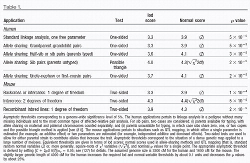 |

Figure 1. Linkage analysis involves constructing a transmission model to explain the inheritance of a disease in pedigrees. The model is straightforward for simple Mendelian traits but can become very complicated for complex traits. Linkage analysis has been applied to hundreds of simple Mendelian traits, as well as to such situations as genetic heterogeneity in breast cancer and two-gene interactions in multiple sclerosis.

Figure 2. Allele-sharing methods involve testing whether affected relatives inherit a region identical-by-descent (IBD) more often than expected under random Mendelian segregation. Affected sib pair analysis is a well-known special case, in which the presence of a trait-causing gene is revealed by more than the expected 50% IBD allele sharing. The method is more robust for genetic complications than linkage analysis but can be less powerful than a correctly specified linkage model. Examples include applications to type I diabetes, essential hypertension, IgE levels, and bone density in postmenopausal women.

Figure 3. Association studies test whether a particular allele occurs at higher frequency among affected than unaffected individuals. Association studies thus involve population correlation, rather than cosegregation within a family. Examples include HLA associations in many autoimmune diseases, apolipoprotein E4 in Alzheimer’s, and angiotension converting enzyme (ACE) in heart disease.

Figure 4. Experimental crosses can provide a large number of progeny while ensuring genetic homogeneity. As a result, experimental crosses permit the genetic dissection of more complex genetic interactions than directly possible in human families, such as mapping of QTLs. Examples include epilepsy in mice, hypertension in rats, type diabetes in mice and rats, and susceptibility to intestinal cancer in mice.
1 A. H. Sturtevant, J. Exp. Zool. 14, 43 (1913).Crossref, Google Scholar
2 W. Bender, P. Spierer, D. S. Hogness, J. Mol. Biol. 168, 17 (1983); P. Spierer, A. Spierer, W. Bender, D. S. Hogness, ibid., p. 35.Crossref, Google Scholar
3 T. D. Petes and D. Botstein, Proc. Natl. Acad. Sci. U.S.A. 74, 5091 (1977).Crossref, Google Scholar
4 D. Botstein, R. L. White, M. H. Skolnick, R. W. Davies, Am. J. Hum. Genet. 32, 314 (1980).Google Scholar
5 D. N. Cooper and J. Schmidtke, Ann. Med. 24, 29 (1992); V. A. McKusick, Mendelian Inheritance in Man: Catalogs of Autosomal Dominant, Autosomal Recessive, and X-Linked Phenotypes (Johns Hopkins Univ. Press, Baltimore, MD, 1992); F. Collins, personal communication.Crossref, Google Scholar
6 T. H. J. Huisman, Am. J. Hematol. 6, 173 (1979); M. H. Steinberg and R. P. Hebbel, ibid. 14,405 (1983).Crossref, Google Scholar
7 G. J. Dover et al., Blood 80, 816 (1992); S. L. Their et al., Am. J. Hum. Genet. 54, 214 (1994).Crossref, Google Scholar
8 D. Easton, D. Ford, J. Peto, Cancer Surv. 18, 95 (1993); D. Ford et al., Lancet 343, 692 (1994).Google Scholar
9 S. T. Reeders et al., Hum. Genet. 76, 348 (1987); G. Romeo et al., Lancet ii, 8 (1988); A. Turco, B. Peissel, L. Gammaro, G. Maschio, P. F. Pignatti, Clin. Genet. 40, 287 (1991).Crossref, Google Scholar
10 P. H. St. George-Hyslop et al., Nature 347, 194 (1990).Crossref, Google Scholar
11 J. Barbosa, H. Noreen, F. C. Goetz, E. J. Yunis, Diabete Metab. 2, 160 (1976); G. I. Bell et al., Proc. Natl. Acad. Sci. U.S.A. 88, 1484 (1991); D. W. Bowden et al., Am. J. Hum. Genet. 50, 607 (1992); P. Froguel et al., Nature 356, 162 (1992).Google Scholar
12 R. Fishel et al., Cell 75, 1027 (1993); F. Leach et al., ibid., p. 1215; N. Papadopoulos et al., Science 263, 1625 (1994); R. Fishel et al., Cell 77, 167 (1994); B. Liu et al., Cancer Res. 54, 4590 (1994).Crossref, Google Scholar
13 N. G. Jaspers and D. Bootsma, Proc. Natl. Acad. Sci. U.S.A. 79, 2641 (1982); E. Sobel et al., Am. J. Hum. Genet. 50, 1343 (1992).Crossref, Google Scholar
14 E. A. De Weerd-Kastelein, W. Keijzer, D. Bootsma, Nat. New Biol. 238, 80 (1972).Crossref, Google Scholar
15 L. M. Bleeker-Wagemakers et al., Genomics 14, 811 (1992); R. Kumar-Singh, P. Kenna, G. J. Farrar, P. Humphries, ibid. 15, 212 (1993).Crossref, Google Scholar
16 S. Brul et al., J. Clin. Invest. 81, 1710 (1988); J. M. Tager et al., Prog. Clin. Biol. Res. 321, 545 (1990); J. Gartner, H. Moser, D. Valle, Nat. Genet. 1, 16 (1992); N. Shimozaun et al., Science 255, 1132 (1992).Crossref, Google Scholar
17 R. Ward, in Hypertension: Pathophysiology, Diagnosis, and Management, J. H. Laragh and B. M. Brenner, Eds. (Raven, New York, 1990), pp. 81–100.Google Scholar
18 W. F. Dietrich et al., Cell 75, 631 (1993).Crossref, Google Scholar
19 K. Kajiwara, E. L. Berson, T. P. Dryja, Science 264, 1604 (1994).Crossref, Google Scholar
20 E. G. Puffenberger et al., Hum. Mol. Genet. 3, 1217 (1994).Crossref, Google Scholar
21 E. S. Lander and D. Botstein, Cold Spring Harbor Symp. Quant. Biol. 51, 49 (1986).Crossref, Google Scholar
22 C. C. Li, Am. J. Hum. Genet. 41, 517 (1987); P. P. Majumder, S. K. Das, C. C. Li, ibid. 43, 119 (1988); S. K. Nath, P. P. Majumder, J. J. Nordlund, ibid., in press.Google Scholar
23 Bilineality has been thought to plague many genetic analyses, particularly those involving psychiatric disorders. See, for example, S. E. Hodge, Genet. Epidemiol. 9, 191 (1992); M. Durner, D. A. Greenberg, S. E. Hodge, Am. J. Hum. Genet. 51, 859 (1992); K. R. Merikangas, M. A. Spence, D. J. Kupfer, Arch. Gen. Psychiatry 46, 1137 (1989); M. A. Spence et al., Hum. Hered. 43, 166 (1993).Crossref, Google Scholar
24 A simple application of the Hardy-Weinberg principle shows that the proportion of individuals who inherit D from a homozygous parent (as opposed to a heterozygous parent) is equal to the allele frequency of D. Suppose that allele D has frequency ρ and let q = 1 − ρ. The proportion of individuals in the population who inherit D from a homozygous parent is 2ρ2/(2ρ2 + 2ρq) = ρ.Google Scholar
25 M. A. Pericak-Vance et al., Am. J. Hum. Genet. 48, 1034 (1991).Google Scholar
26 E. H. Corder et al., Science 261, 921 (1993).Crossref, Google Scholar
27 D. C. Wallace, Annu. Rev. Biochem. 61, 1175 (1992); J. B. Redman, R. G. Fenwick Jr., Y. H. Fu, A. Pizzuti, C. T. Caskey, J. Am. Med. Assoc. 269, 1960 (1993).Crossref, Google Scholar
28 N. J. Schork and S. W. Guo, Am. J. Hum. Genet. 53, 1320 (1993).Google Scholar
29 M. J. Khoury, T. H. Beaty, B. H. Cohen, Fundamentals of Genetic Epidemiology (Oxford Univ. Press, New York, 1993); K. M. Weiss, Genetic Variation and Human Disease (Cambridge Univ. Press, Cambridge, 1993).Google Scholar
30 M. C. Neale and L. R. Cardon, Methodology for Genetic Studies of Twins and Families (Kluwer Academic, Boston, 1992).Google Scholar
31 L. S. Penrose, Acta Genet. 4, 257 (1953); J. H. Edwards, ibid. 10, 63 (1960); Br. Med. Bull. 25, 58 (1969); N. Risch, Am. J. Hum. Genet. 46, 222 (1 990).Google Scholar
32 N. Risch, Am. J. Hum. Genet. 46, 229 (1990).Google Scholar
33 ———, ibid., p. 242.Google Scholar
34 The concept of heritability has a long history in genetics, being one of the most widely used terms in all of biology; see, for example, R. A. Fisher, Trans. R. Soc. Edinburgh 52, 399 (1918); D. S. Falconer, Introduction to Quantitative Genetics (Longman, New York, 1981).Crossref, Google Scholar
35 B. Newman, M. A. Austin, M. Lee, M. C. King, Proc. Natl. Acad. Sci. U.S.A. 85, 3044 (1988).Crossref, Google Scholar
36 See also W. R. Williams and D. E. Anderson, Genet. Epidemiol. 1, 7 (1984); D. T. Bishop, L. Cannon-Albright, T. McLellan, E. J. Gardner, M. H. Skolnick, Genet. Epidemiol. 5, 151 (1988); E. B. Claus, N. J. Risch, W. D. Thompson, Am. J. Epidemiol. 131, 961 (1990).Crossref, Google Scholar
37 Problems that arise through the ascertainment of probands whose families are then used in genetic studies have been discussed at length in the genetics literature. Some articles of relevance are W. Weinberg, Arch. Rassen-Gesellschaftsbiol. 9, 165 (1912); N. E. Morton, Am. J. Hum. Genet. 11, 1 (1959); W. J. Ewens, ibid. 34, 853 (1982); P. P. Majumder, Stat. Med. 4,163 (1985); W. J. Ewens and N. C. Shute, Ann. Hum. Genet. 50, 399 (1986); M. R. Young, M. Boehnke, P. P. Moll, Am. J. Hum. Genet. 43, 705 (1988).Google Scholar
38 J. Ott, Am. J. Hum. Genet. 46, 219 (1990).Google Scholar
39 The number of major genetic factors segregating in a cross between inbred strains can be estimated under some circumstances; see (47); W. E. Castle, Science 54, 223 (1916); S. Wright, Evolution and the Genetics of Populations: Genetic and Biometric Foundations (Univ. of Chicago Press, Chicago, 1968), pp. 373– 420.Google Scholar
40 M. W. Feldman and L. L. Cavalli-Sforza, in Genetic Aspects of Common Diseases: Applications to Predictive Factors in Coronary Disease (Liss, New York, 1979), pp. 203–227.Google Scholar
41 K. W. Kinzier et al., Science 253, 661 (1991); G. Joslyn et al., Cell 66, 601 (1991).Crossref, Google Scholar
42 L. A. Aaltonen et al., Science 260, 812 (1993).Crossref, Google Scholar
43 R. R. Williams et al., Arch. Intern. Med. 150, 582 (1990); J. V. Selby et al., J. Am. Med. Assoc. 265, 2079 (1991); R. R. Williams et al., Ann. Med. 24, 469 (1992).Crossref, Google Scholar
44 R. F. Clark and A. M. Goate, Arch. Neurol. 50, 1164 (1993).Crossref, Google Scholar
45 M. E. Marenberg, N. Risch, L. F. Berkman, B. Floderus, U. de Faire, N. Engl. J. Med. 330, 1041 (1994).Crossref, Google Scholar
46 G. Carey and J. Williamson, Am. J. Hum. Genet. 49, 786 (1991); L. R. Cardon and D. W. Fulker, Am. J. Hum. Genet., in press; N. J. Schork et al., in preparation.Google Scholar
47 E. S. Lander and D. Botstein, Genetics 121, 174 (1989).Google Scholar
48 L. Groop and R. DeFranzo, personal communication.Google Scholar
49 G. A. Barnard, R. Stat. Soc. J. B11, 115 (1949); J. B. S. Haldane and C. A. B. Smith, Ann. Eugen. 14, 10 (1947); J. Chotoi, Ann. Hum. Genet. 48, 359 (1984).Google Scholar
50 N. E. Morton, Am. J. Hum. Genet. 8, 80 (1955).Google Scholar
51 A. W. F. Edwards, Likelihood (Johns Hopkins Univ. Press, Baltimore, MD, 1992).Google Scholar
52 J. Ott, Analysis of Human Genetic Linkage (Johns Hopkins Univ. Press, Baltimore, MD, 1991), pp. 65– 68.Google Scholar
53 J. Tomfohrde et al., Science 264, 1141 (1994).Crossref, Google Scholar
54 J. K. Ghosh and P. K. Sen, in The Proceedings of the Berkeley Conference in Honor of Jerzy Neyman and Jack Kiefer, L. M. LeCam and R. A. Olshen, Eds. (Wadsworth, Monterey, CA, 1985), pp. 807– 810; D. M. Titterington, A. F. M. Smith, U. E. Makov, Statistical Analysis of Finite Mixture Distributions (Wiley, London, 1985); J. Ott, in (52), pp. 194–216; J. Faraway, Genet. Epidemiol. 10, 75 (1993); H. Chernoff and E. S. Lander, J. Stat. Plann. Inference, in press.Google Scholar
55 J. M. Hall et al., Science 250, 1684 (1990).Crossref, Google Scholar
56 G. D. Schellenberg et al., ibid. 258, 668 (1992); C. E. Yu et al., Am. J. Hum. Genet. 54, 631 (1994).Google Scholar
57 R. Sherrington et al., Nature 336, 164 (1988).Crossref, Google Scholar
58 E. S. Lander and D. Botstein, Proc. Natl. Acad. Sci. U.S.A. 83, 7353 (1986); N. J. Schork, M. Boehnke, J. D. Terwilliger, J. Ott, Am. J. Hum. Genet. 53, 1127 (1993).Crossref, Google Scholar
59 C. S. Haley and S. A. Knott, Heredity 69, 315 (1992).Crossref, Google Scholar
60 P. J. Tienari et al., Genomics 19, 320 (1994).Crossref, Google Scholar
61 D. E. Weeks, T. Lehner, E. Squires-Wheeler, C. Kaufmann, J. Ott, Genet. Epidemiol. 7, 237 (1990).Crossref, Google Scholar
62 One way of avoiding the possible use of an incorrectly specified segregation model in a linkage analysis is to estimate linkage and segregation parameters simultaneously. Although computationally prohibitive in certain settings, this strategy appears to have some favorable features. See, for example, C. J. MacLean, N. E. Morton, S. Yee, Comput. Biomed. Res. 17, 471 (1984); G. E. Bonney, G. M. Lathrop, J. M. Lalouel, Am. J. Hum. Genet. 43, 29 (1988); N. J. Schork, Genet. Epidemiol. 9, 207 (1992).Crossref, Google Scholar
63 J. Ott, Clin. Genet. 12, 119 (1977); F. Clerget-Darpoux, Ann. Hum. Genet. 46, 363 (1982); ______, C. Bonaiti-Pellie, J. Hochez, Biometrics 42, 393 (1986); F. Clerget-Darpoux, M. C. Babron, C. Bonaiti-Pellie, J. Psychiatr. Res. 21, 625 (1987).Google Scholar
64 For a discussion of how robust linkage analysis might be in certain settings, see, for example, J. A. Williamson and C. I. Amos, Genet. Epidemiol. 7, 309 (1990); C. I. Amos and J. A. Williamson, Am. J. Hum. Genet. 52, 213 (1993); S. E. Hodge and R. C. Fiston, Genet. Epidemiol., in press.Crossref, Google Scholar
65 L. J. Eaves, Heredity 72, 175 (1994).Crossref, Google Scholar
66 J. Ott, Am. J. Hum. Genet. 31, 161 (1979); J. Edwards, Cytogenet. Cell Genet. 39, 43 (1982); N. J. Schork, in Computing Science and Statistics: Proceedings of the 23rd Symposium on the Interface, Seattle, WA, 21–24 April 1994, E. M. Keramidas and S. M. Kaufman, Eds. (Interface Foundation of North America, Fairfax Station, VA, 1992); T. M. Goradia, K. Lange, P. L. Miller, P. M. Nadkarni, Hum. Hered. 42, 42 (1992); R. W. Cottingham Jr., R. M. Idury, A. A. Schaffer, Am. J. Hum. Genet. 53, 252 (1993).Google Scholar
67 N. J. Schork, Genet. Epidemiol. 8, 29 (1991).Crossref, Google Scholar
68 R. C. Elston and J. Stewart, Hum. Hered. 21, 323 (1971).Google Scholar
69 Since its introduction, the Elston-Stewart algorithm has been extended and modified in various ways; see, for example, J. Ott, Am. J. Hum. Genet. 26, 588 (1974); K. Lange and R. C. Elston, Hum. Hered. 25, 95 (1975); C. Cannings, E. T. Thompson, M. H. Skolnick, Adv. Appl. Probab. 10, 26 (1978); R. C. Elston, V. T. George, F. Severtson, Hum. Hered. 42,16 (1992).Google Scholar
70 J. Ott, Am. J. Hum. Genet. 28, 528 (1976).Google Scholar
71 G. M. Lathrop, J. M. Lalouel, C. Julier, J. Ott, Proc. Natl. Acad. Sci. U.S.A. 81, 3443 (1984).Crossref, Google Scholar
72 N. E. Morton and C. J. MacLean, Am. J. Hum. Genet. 26, 489 (1974); S. J. Hasstedt, Comput. Biomed. Res. 15, 295 (1982); G. E. Bonney, Am. J. Med. Genet. 18, 731 (1984); S. W. Guo and E. T. Thompson, IMA J. Math. Appl. Med. Biol. 8, 171 (1991); ibid., p. 149; N. J. Schork, Genet. Epidemiol. 9, 73 (1992).Google Scholar
73 M. C. King, G. M. Lee, N. B. Spinner, G. Thompson, M. R. Wrensch, Annu. Rev. Public Health 5, 1 (1984); E. A. Thompson, Stat. Med. 5, 291 (1986).Crossref, Google Scholar
74 E. S. Lander and P. Green, Proc. Natl. Acad. Sci. U.S.A. 84, 2363 (1987).Crossref, Google Scholar
75 L. Kruglyak and E. S. Lander, in preparation.Google Scholar
76 S. W. Guo and E. T. Thompson, Am. J. Hum. Genet. 51,1111 (1992); D. C. Thomas, Cytogenet. Cell Genet. 59, 228 (1992); A. Kong, N. Cox, M. Frigge, M. Irwin, Genet. Epidemiol. 10, 483 (1993).Google Scholar
77 For a discussion, see W. C. Blackwelder and R. C. Elston, Genet. Epidemiol. 2, 85 (1985); A. S. Whittemore and J. Halpern, Biometrics 50, 118 (1994).Crossref, Google Scholar
78 D. E. Weeks and K. Lange, Am. J. Hum. Genet. 42, 315 (1988).Google Scholar
79 B. K. Suarez, J. Rice, T. Reich, Ann. Hum. Genet. 42, 87 (1978).Crossref, Google Scholar
80 L. R. Weitkamp, N. Engl. J. Med. 305, 1301 (1981); M. Knapp, S. A. Beuchter, M. P. Baur, Hum. Hered. 44, 37 (1994).Crossref, Google Scholar
81 P. Holmans, Am. J. Hum. Genet. 52, 362 (1993).Google Scholar
82 N. E. Morton et al., ibid. 35, 201 (1983); R. N. Hyer et al., ibid. 48, 243 (1991); S. S. Rich, S. S. Panter, F. C. Goetz, B. Hedlund, J. Barbosa, Diabetologica 34, 350 (1991).Google Scholar
83 D. Owerbach and K. H. Gabbay, Am. J. Hum. Genet. 54, 909 (1994).Google Scholar
84 J. Davies et al., Nature, in press.Google Scholar
85 D. H. Hamer, S. Hu, V. L. Magnuson, N. Hu, A. M. L. Pattatucci, Science 261, 321 (1993).Crossref, Google Scholar
86 In principle, one could either explicitly use the expected value of the IBD statistic or work with the probability distribution over the IBD statistic. The former approach has the difficulty that it is hard to derive an expression for the variance of the statistic. It has been done in some simple cases, such as inbred crosses (L. Kruglyak and E. S. Lander, submitted). The latter has been applied in numerous cases [for example, (79); C. I. Amos, D. V. Dawson, R. C. Elston, Am. J. Hum. Genet. 47, 842 (1990)].Google Scholar
87 K. Lange, Am. J. Hum. Genet. 39, 148 (1986); D. E. Weeks and K. Lange, ibid. 50, 859 (1992).Google Scholar
88 X. Jeunemaitre et al., Cell 71, 169 (1992).Crossref, Google Scholar
89 J. K. Haseman and R. C. Elston, Behav. Genet. 2, 3 (1972).Crossref, Google Scholar
90 W. C. Blackwelder and R. C. Elston, Commun. Stat. Theor. Methods 11, 449 (1982); C. I. Amos and R. C. Elston, Genet. Epidemiol. 6, 349 (1989); J. M. Olson and E. M. Wijsman, ibid. 10, 87 (1993).Crossref, Google Scholar
91 C. I. Amos et al., Genet. Epidemiol. 3, 255 (1986).Crossref, Google Scholar
92 D. G. Marsh et al., Science 264, 1152 (1994).Crossref, Google Scholar
93 N. A. Morrison et al., Nature 367, 284 (1994).Crossref, Google Scholar
94 0. F. Goldgar, Am. J. Hum. Genet. 47, 957 (1990); C. I. Amos, ibid. 54, 535 (1994); D. W. Fulker and L. R. Cardon, ibid., p. 1092; N. J. Schork and S. Ghosh, submitted.Google Scholar
95 W. H. Berrittini et al., Proc. Natl. Acad. Sci. U.S.A. 91, 5918 (1994).Crossref, Google Scholar
96 L. P. Ryder, E. Andersen, A. Svejgaard, Eds., HLA and Disease Registry, Third Report (Munksgaard, Copenhagen, 1979).Google Scholar
97 W. E. Braun, HLA and Disease (CRC, Boca Raton, FL, 1979).Google Scholar
98 E. H. Corder et al., Nat. Genet. 7, 180 (1994); C. Singer et al., Arch. Neurol. 49, 13 (1992); F. Schachter et al., Nat. Genet. 6, 29 (1994); H. Schunkert et al., N. Engl. J. Med. 330, 1634 (1994); F. Cambien et al., Nature 359, 641 (1992).Crossref, Google Scholar
99 Some of these methods have generally fallen under the heading of “measured genotype” analyses. Relevant articles include E. Boerwinkle, R. Chakraborty, C. F. Sing, Ann. Hum. Genet. 50,181 (1986); V. T. George and R. C. Elston, Genet. Epidemiol. 4, 193 (1987).Crossref, Google Scholar
100 An exception would be if there were so many disease-causing alleles that the association could not be easily detected, or if the trait were predominantly due to a different cause in some populations.Google Scholar
101 This could happen if the ancestral disease-causing chromosome carried both the Eco RI and the Bam HI sites, but many normal chromosomes also had the Eco RI site but not the Bam HI site.Google Scholar
102 K. M. Weiss, Genetic Variation and Human Disease (Cambridge Univ. Press, Cambridge, 1993).Google Scholar
103 C. T. Falk and P. Rubinstein, Ann. Hum. Genet. 51, 227 (1987); F. Clerget-Darpoux et al., ibid. 52, 247 (1988); G. Thompson et al., Genet. Epidemiol. 6, 43 (1989); J. Ott, ibid., p. 127; J. D. Terwilliger and J. Ott, Hum. Hered. 42, 337 (1992); M. Knapp, S. A. Seuchter, M. P. Baur, Am. J. Hum. Genet. 52, 1085 (1993).Crossref, Google Scholar
104 C. Julier et al., Nature 354, 155 (1991).Crossref, Google Scholar
105 R. S. Spielman et al., Am. J. Hum. Genet. 52, 506 (1993); S. E. Hodge, ibid. 53, 367 (1993).Google Scholar
106 K. Blum et al., J. Am. Med. Assoc. 263, 2055 (1990).Crossref, Google Scholar
107 J. Gelemnter et al., ibid. 266, 1801 (1991); K. Blum et al., Alcohol 10, 59 (1993); J. Gelernter et al., J. Am. Med. Assoc. 269, 1673 (1993).Crossref, Google Scholar
108 D. Goldman et al., Alcohol. Clin. Exp. Res. 17, 199 (1993); B. K. Suarez et al., Genomics 19, 12 (1994); C. N. Pato et al., Am. J. Med. Genet. 48, 78 (1993); A. Parsian et al., Arch. Gen. Psychiatry 48, 655 (1991); T. Arinami et al., Biol. Psychiatry 33, 108 (1993); D. Goldman et al., Acta Psychiatr. Scand. 86, 351 (1992); S. Schwab et al., Am. J. Hum. Genet. 49 (suppl.), 203 (1991); D. Goldman et al., Alcohol. Clin. Exp. Res., in press.Crossref, Google Scholar
109 Indeed, a perfect association between two loci linked at 1% recombination decays with a “half-life” of about 70 generations, because (0.99)70 ≈1/2. This corresponds to about 1500 years for humans.Google Scholar
110 R. Plomin et al., Behav. Genet. 24, 107 (1994).Crossref, Google Scholar
111 R. Chakraborty and K. M. Weiss, Proc. Natl. Acad. Sci. U.S.A. 85, 9119 (1988).Crossref, Google Scholar
112 QTL analysis is included under the heading of polygenic trait analysis, despite the fact that a quantitative trait could, in principle, be monogenic. In practice, quantitative traits are nearly always polygenic, and the methodology is the same in any case.Google Scholar
113 H. Jacob, Cell 67, 213 (1991).Crossref, Google Scholar
114 T. Serikawa et al., Genetics 131, 701 (1992).Google Scholar
115 E. A. Carbonell, T. M. Gerig, E. Balansard, M. J. Asins, Biometrics 48, 305 (1992); Z. W. Luo and M. J. Kearsey, Heredity 69, 236 (1992); Z. B. Zeng, Genetics 136, 1457 (1994); S. A. Knott and C. S. Haley, ibid. 132, 1211 (1992); R. C. Jansen and P. Stam, ibid. 136, 1447 (1994); Z. B. Zeng, Proc. Natl. Acad. Sci. U.S.A. 90, 10972 (1993); R. C. Jansen, Genetics 135, 205 (1993); Theor. Appl. Genet. 85, 252 (1992).Crossref, Google Scholar
116 Work on gene-mapping schemes in experimental organisms is ongoing and a topic of great interest in statistical genetics. For example, L. Kruglyak and E. S. Lander (submitted) have developed a nonparametric method for QTL mapping; N. J. Schork (submitted) has shown how to use interval mapping for dichotomous traits; and N. J. Schork (submitted) has described methods for detecting epistatic interaction.Google Scholar
117 The key reason is that the meioses in experimental crosses are all equivalent (that is, they involve segregation of the same alleles in a fixed phase relationship, with each parent being heterozygous for a “high” and “low” allele at a QTL in, for example, F2 progeny), whereas the meioses in different human families are not directly comparable (that is, the configuration of “high” and “low” alleles varies among each set of parents, and only a subset of parents segregate for different alleles at a QTL). Accordingly, QTL analysis in experimental crosses allows one to compare means (for example, the mean phenotype of progeny inheriting allele A versus the mean phenotype of progeny inheriting allele B), whereas QTL analysis of human families requires one to compare variances (for example, squared differences Δ2 between sib pairs inheriting two IBD alleles versus between sib pairs inheriting no alleles IBD, as in the Haseman-Elston method).Google Scholar
118 P. C. Groot et al., FASEB J. 6, 2826 (1992); C. J. Moen, M. Snoek, A. A. Hart, P. Demant, Oncogene 7, 563 (1992).Crossref, Google Scholar
119 A. H. Paterson et al., Nature 335, 721 (1988).Crossref, Google Scholar
120 M. L. Rise, W. N. Frankel, J. M. Coffin, T. N. Seyfried, Science 253, 669 (1991); P. Hilbert et al., Nature 353, 521 (1991).Crossref, Google Scholar
121 S. D. Tanksley, Annu. Rev. Genet. 27, 205 (1993); J. C. Crabbe, J. K. Belknap, K. J. Buck, Science 264, 1715 (1994).Crossref, Google Scholar
122 M. Festing, Inbred Strains in Biomedical Research (Oxford Univ. Press, New York, 1979).Google Scholar
123 S. Ghosh et al., Nat. Genet. 4, 404 (1993); N. Risch, S. Ghosh, J. A. Todd, Am. J. Hum. Genet. 53, 702 (1993).Crossref, Google Scholar
124 H. J. Jacob et al., Nat. Genet. 2, 56 (1992).Crossref, Google Scholar
125 J. A. Egeland et al., Nature 325, 783 (1987); J. L. Kennedy et al., ibid. 336, 167 (1988); S. D. Detera-Wadleigh et al., ibid. 340, 391 (1989); J. R. Kelsoe et al., ibid. 342, 238 (1989); M. Baron et al., Nat. Genet. 3, 49 (1993).Crossref, Google Scholar
126 E. Feingold, P. 0. Brown, D. Siegmund, Am. J. Hum. Genet. 53, 234 (1993).Google Scholar
127 The factor [C + 2ρGh(T)] approximately converts a single-point significance level aT to a genome-wide significance level αT*, both for lod scores and allelesharing statistics. The factor is asymptotically correct for large values of T and thus small values of αT and αT*. The significance-level αT can also be regarded as the expected number of distinct regions in which the statistic X exceeds T. The significance level can be one-sided or two-sided. For a normally distributed statistic, h(T) = T2. For a lod score statistic, h(T) = T(2loge10). The constant ρ measures the crossover rate. If R(d) denotes the covariance function between genotypes (or allele-sharing status) at distance d (measured in Morgans), then ρ is defined by the equation ρ= − R′ (0)/2, where R′ (0) denotes the derivative at zero taken as a limit from above. In the simple case of individual informative meioses in a nuclear family or a single-generation cross, R(d) = exp(−2d). More generally, R(d) is of the form a1exp(−b1d) + a2exp(−b2d) +… + akexp(−bkd). For example, first-cousin allele sharing has R(d) = exp(−4d)/2 + exp(−6d)/3 + exp(−8d)/6. One can show that ρ = 1 for backcrosses or intercrosses in which only an additive component is fit (1 df); ρ= 1.5 for intercrosses in which an additive and dominance component is fit (2 df); ρ= 1 for grandparent-grandchild pair allele sharing; ρ= 2 for half-sib pair allele sharing (as well as for sib pairs regarded as the sum of two half-sib pairs) and for recombinant inbred lines produced by selfing; ρ= 2.5 for uncle-nephew pair allele sharing; ρ= 8/3 for first-cousin pair allele sharing; and ρ= 4 for recombinant inbred strains produced by brother-sister mating. The analysis has also been modified by D. Siegmund (personal communication) for sib pair allele sharing in which the significance test is based on the possible triangle method (81). The calculated values in Table 1 are from L. Kruglyak, D. Siegmund, E. S. Lander, in preparation.Google Scholar
128 A. Rebai, B. Goffinet, B. Mangin, Genetics 138, 235 (1994); W. N. Frankel et al., ibid., in press.Google Scholar
129 K. K. Kidd and J. Ott, Cytogenet. Cell Genet. 37, 510 (1984).Google Scholar
130 J. Ott, Proc. Natl. Acad. Sci. U.S.A. 86, 4175 (1989); J. D. Terwilliger and J. Ott, Cytogenet. Cell Genet. 59, 142 (1992); M. N. Chiano and J. R. W. Yates, Ann. Hum. Genet. 58, 129 (1994); N. J. Schork, in Exploring the Limits of the Bootstrap, R. LePage and L. Billard, Eds. (Wiley, New York, 1991); and M. A. Schork, Am. J. Hum. Genet. 45, 803 (1989); A. Kong, M. Frigge, M. Irwin, N. Cox, ibid. 51, 1413 (1992).Crossref, Google Scholar
131 To illustrate the flexibility of permutation tests, suppose that a genome scan detects two loci on chromosomes 1 and 2 that appear to affect a trait in an additive fashion, with the first explaining twice as much variance as the second. To determine whether the second locus makes a significant contribution over and above the first, one could permute the genotypes for chromosome 2 among the progeny. The likelihood ratio statistic for a two-locus effect can be computed for each such permutation and the empirical distribution used to make inferences about the significance of the effect of the second locus.Google Scholar
132 See, for example, E. S. Edgington, Randomization Tests (Dekker, New York, 1987); E. W. Noreen, Computer Intensive Methods for Testing Hypotheses (Wiley, New York, 1989); B. Efron and R. J. Tibshirani, An Introduction to the Bootstrap (Chapman & Hall, New York, 1994), pp. 220–236.Google Scholar
133 J. K. Belknap, Behav. Genet. 22, 677 (1992).Crossref, Google Scholar
134 Informative meioses are those in which one can definitively tell if the disease-causing allele has been transmitted from an obligate heterozygote. For a fully penetrant monogenic dominant trait, all meioses occurring in an affected individual are informative. For a fully penetrant monogenic recessive trait, meioses occurring in an obligate carrier are informative if they produce an affected child or if they produce an unaffected child who inherits the disease-causing allele from the other parent. This latter situation occurs in one-third of unaffected children and can be recognized by the use of close flanking markers.Google Scholar
135 M. Boehnke, Am. J. Hum. Genet. 39, 513 (1986); D. E. Weeks, J. Ott, G. M. Lathrop, ibid. 47, A204 (1990).Google Scholar
136 D. Brown, M. B. Gorin, D. E. Weeks, ibid. 54, 544 (1994).Google Scholar
137 C. Cannings and E. T. Thompson, Clin. Genet. 12, 208 (1977); M. Boehnke, M. R. Young, P. P. Moll, Am. J. Hum. Genet. 43, 336 (1988); A. E. Pulver et al., Am. J. Med. Genet. 54, 36 (1994); E. A. Thompson, Theor. Popul. Biol. 24, 39 (1983); Am. J. Hum. Genet. 33, 968 (1981); Biometrics 37, 313 (1981); M. Boehnke, K. H. Omoto, J. M. Arduino, Am. J. Hum. Genet. 46, 581 (1990). In cases involving a disease-causing allele D with high frequency, one may also wish to avoid families with “too many” affected individuals, because there is a high probability that one or both parents is homozygous for D (L. Kruglyak and E. S. Lander, in preparation).Google Scholar
138 J. S. Beckman, in Gene Mapping Techniques and Applications, L. B. Schook, H. A. Lewin, D. G. McLaren, Eds. (Dekker, New York, 1991), pp. 201–229.Google Scholar
139 D. T. Bishop and J. A. Williamson, Am. J. Hum. Genet. 46, 254 (1990).Google Scholar
140 A. Darvasi, A. Weinreb, V. Minke, J. I. Weller, M. Soller, Genetics 134, 943 (1993); Z. B. Zeng, ibid. 136, 1457 (1994).Google Scholar
141 R. C. Elston, in Proceedings of the 16th International Biometric Conference, Hamilton, New Zealand, 7–11 December 1992 (Ruakura Conference Center, Hamilton, New Zealand, 1992), pp. 39–51.Google Scholar
142 Crossovers are randomly distributed with density N per centimorgan, where N is the number of informative meioses. It follows trivially that the expected distance to the nearest flanking crossover on either side is (1/N) cM. [See also, K. Lange, L. Kunkel, J. Aldridge, S. A. Latt, Am. J. Hum. Genet. 37, 853 (1985); M. Boehnke, ibid. 55, 379 (1994).]Google Scholar
143 J. Hastbacka et al., Cell 78, 1073 (1994).Crossref, Google Scholar
144 N. Risch, Am. J. Hum. Genet. 53 (suppl.), abstract 185 (1993); L. Kruglyak and E. S. Lander, submitted.Google Scholar
145 B. Kerem et al., Science 245, 1073 (1989); J. Hastbacka et al., Nat. Genet. 2, 204 (1992).Crossref, Google Scholar
146 In a population founded N generations ago, linkage disequilibrium should be detectable over distances on the order of (100/N) cM. By studying k affected chromosomes, one should be able to localize a disease gene to a region on the order of (100/kN)) cM. (Exact numbers would depend on the precise definition of detection of linkage disequilibrium and localization of a disease gene, but these estimates reflect the scaling with population age and number of affected chromosomes.)Google Scholar
147 Traditional construction of congenic strains by repeated backcrossing relies on the fact that an average of 50% of the undesired genome is lost at each generation. By using a complete genetic linkage map, however, one can identify those backcross progeny that have fortuitously lost a larger proportion of the undesired genome and breed them to create the next generation. In only three to four generations, it is possible to eliminate essentially all of the undesired genome. For example, this has been performed to construct congenic strains for the Mom-1 region of mouse chromosome 4 (A. Moser and W. F. Dietrich, personal communication).Google Scholar
148 Complementation tests can be performed only between two alleles causing the same recessive phenotype. Accordingly, knockout experiments should target an allele A1 that causes a dominant (or partially dominant) phenotype when placed in trans to a second allele A2; the knockout allele would then be expected to fail to yield the dominant phenotype in the complementation test. Because current gene knockout protocols are limited to a few mouse strains such as 129, one may first need to construct a congenic carrying the desired allele in such a strain before one can construct the appropriate knockout.Google Scholar
149 For an insightful historical account of the criticisms of Mendelian theory on the grounds that it cannot explain variation observed in nature, see W. B. Provine, The Origins of Theoretical Population Genetics (Univ. of Chicago Press, Chicago, 1971).Google Scholar
150 We thank L. Kruglyak and D. Siegmund for assistance concerning thresholds for significance and C. Amos, M. Boehnke, A. Chakravarti, F. Collins, R. Elston, W. Frankel, D. Fulker, S. Ghosh, S.-W. Guo, H. Jacob, J. Ott, A. Weder, A. Lynn, and members of the Lander laboratory for helpful comments on the manuscript. This work was supported in part by a grant from NIH (HG00098 to E.S.L.).Google Scholar

